Custom formats in Excel

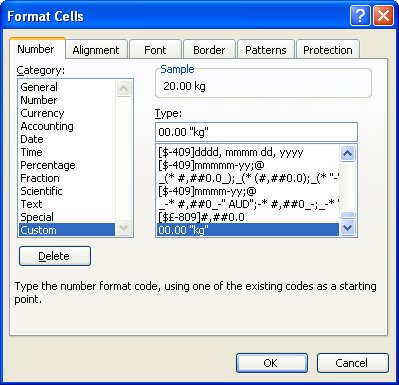
Ok, so here's the scenario, you want to enter a value like 20Kg (or 44 lb) into an Excel cell. All goes well until you try to multiply the value. Instant disaster. Your number isn't a number it's a piece of text and you can't multiply or add text. You can't divide or minus text or find the 4th power of it either - you get the idea.. it's basically a useless entry - pretty but useless.

SO, how do you format a cell so it displays the Kg after the number but so it still treats the entry as a number? I'm so glad you asked!

The answer is to create a custom number format. Click the cell or a range of cells and choose Format > Cells > Number tab. Select the Custom entry and type something like 00.00 "kg" in the text box and click Ok. Now, enter the numbers again as 20 or 40 etc and the kg will appear automatically after the number courtesy of the format - and the number, well it's still a number so you can add, multiply, divide and do all sorts of other wonderful things to it as you like.

You can also add the text before a number. So, for all those lovely Canada dollars I get paid by the folk at Hub Digital Living where I write a monthly Office column, I type a Custom format like "CAN" 00.00 in my sheet where I record my payments. It's all so easly when you know how.. and now - you do too..

Converting Imported data in Excel

I encountered an interesting problem with Excel this morning when I tried to import data copied from a table in a PDF file. The table was bad news from my accountant about my retirement investments. I won't be retiring any time soon ;)

The point of the issue however was that the data when copied and pasted into Excel came in neatly aligned in column but the numbers wouldn’t add up because they’d been added as text.

The solution to this is to use a feature previously called data parsing. What it does is to look at the data and convert it from one format to another. My only alternative would have been to select each cell, double-click on the cell to get the number on the screen, remove any characters that were causing issues such as any leading dollar signs or spaces and then press Enter to convert the text value into a number.

Luckily data parse does the work for you almost instantly. To do this, select the column of numbers that you’re working on. If you have a whole lot of columns to do, you still have to do each column one at a time. That’s the bad news; the rest of it is all good.

Select the column of numbers (if it includes some text entries that doesn’t matter), choose Data > Text to Columns and then select Delimited as the Original Data Type and click Next.

Click Next again and this is where you get to do the work. To convert text to numbers select the General option. If you have dates then select the Date option and select the date format that the data was created in. My values came from Australia so the date format used was dd-mmm-yy. Provided you select the date format that matches the dates you have, everything will convert just fine. Later if you want to show these in another format such as mm-dd-yy you do so using a date format. When you’re done, just click Finish.

The data will be instantly converted and you can move forward to do the same thing on the next column.

I estimate that this process took me about three minutes to do and on the data that I had it could have taken me half an hour or more to fix it all manually.

So next time you’ve imported data from an external source and when you need to convert text back into numbers check out the Data > Text in Columns option.

Change spelling wavy underline color

Ok, so this post can happily be filed in the "Gee I really needed to know that - NOT!" category. It's seriously fun but, unless you're color blind, not something you absolutely HAVE to know.

It's easy (if you're a dab hand at changing registry entries) to change the color of the wavy underlines used for spelling and grammar errors in Word 2007. Choose Start > Run > Regedit and locate this key:

HKEY_CURRENT_USER\Software\Microsoft\Shared Tools\Proofing Tools

If the SpellingWavyUnderlineColor entry exists, double-click it and when the Edit DWORD value dialog appears, click Hexadecimal and type an eight digit hexadecimal number representing the RGB color value of the color to use (add two leading zeros to the value). So to use Blue, type 000000FF and click Ok. If the value isn't in the list, choose Edit > New > DWORD value, type SpellingWavyUnderlineColor and then double-click it and change its DWORD value to the hexadecimal number you want to use.

To change the grammar underline color, change the GrammarWavyUnderlineColor value, and to change the contextual spelling error color change the ContextualSpellingWavyUnderlinecolor entry. If any entries don't exist, just create them.

When you're done, close the registry, restart the computer, and restart Word and the changes will be in place.

If you don't know what hexadecimal color is what, visit http://www.patman.org/webdesign/hexcolors2.asp and find a color and its appropriate hexadecimal value here. Add two leading zeros and you're done.

Of course, before you touch the Registry you should back it up in case everything goes pear shaped. Also - NEVER mess with anything you don't understand!