Excel 2007- In Cell Dropdown List

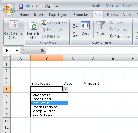
When you need to enter data from a small subset of entries into a range in Excel 2007 you can do it more easily using a custom designed dropdown list.

To configure a dropdown list in a cell type the list of items to use in a single column in a spare sheet in the workbook.

Select these cells and choose the Formulas tab Define Name, type DataForList as the name in the dialog, set the scope to Workbook and click Ok.

Switch to the sheet where you want to add your dropdown list to some cells, select the cells that should display a list of data to choose from and choose Data tab > Data Validation > Settings tab.

From the Allow: dropdown list choose List and, in the Source area, type =DataForList and click Ok.

Now, whenever you click a cell in this range you’ll see a dropdown list appear from which you can choose a list entry for that cell.

If you're using Excel 2003, here is a link to an earlier post explaining how to do this in Excel 2003:

Automatic cell entries in Excel 2003
http://www.projectwoman.com/labels/validation.html

Excel: Print a worksheet your way

When you need to print one version of a worksheet for yourself and another for the boss and you like it small and he likes it to be - well just how he likes it, then you need Views. The Excel Views tool lets you configure a worksheet for different printing options and to save these so you can use them again later on.

You can set views up so you do one for your boss and one for you. Or, you can set one up to print only the summary part of a worksheet and another to print the lot. Even if the print areas and the print settings change, Views let you preconfigure them so you don’t have to set them up manually every time. Better still, Views are saved with the worksheet so they're always available.

Step 1
To save a set of printing settings, first set up your worksheet with the print settings you want to use including setting a print area if needed.

Step 2
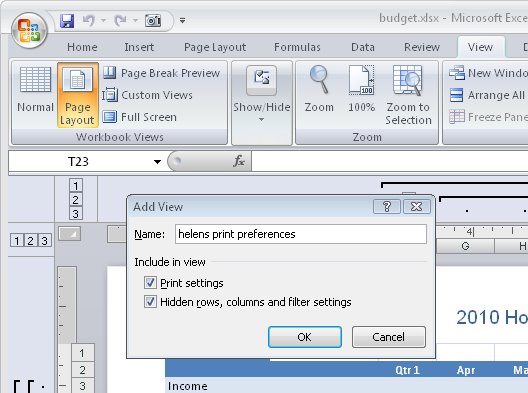
To save this set up, choose View > Custom Views > Add (in Excel 2007 choose the View tab > Custom Views > Add). Type a name for the view that explains what settings you have selected. Enable the Print Settings checkbox and click Ok. You can now create another view and save it. Do this for as many different settings as you need. Save your worksheet.

Step 3
In future, before you print, choose View > Custom Views > select the View you want to use and click Show. Now go and print the worksheet - your settings were saved so you don't need to configure them.

Excel page headers and footers

When you're printing a 50 page worksheet, you want to hold onto the printed pages very carefully. If you don't the entire project is prone to disaster as it is all too easy for the pages to get out of order and it’s nearly impossible to sort out the mess. So, either staple them very quickly or use the header and footer tool in Excel to add page numbers to all your pages.

Of course, while page numbers are one of the most common things you might put in a header or footer it isn't the only thing. You can add everything from the date to your company’s logo.

To add a header or footer that will print on every page of an Excel workbook, choose View > Header and Footer in Excel 2003 or, in Excel 2007 choose Insert tab > Header & Footer. In Excel 2003 you can select from a range of preset headers and footers which are configured using typical combinations of items usually used in headers or footers – for example, sheet and worksheet names, page numbers, filename and folders.

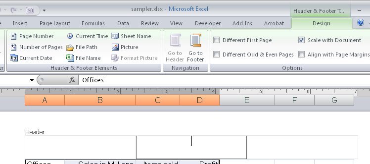
If you'd prefer to create your own headers and footers, click the Custom Header or Custom Footer button and create your own design - this is the way you create a header or footer in Excel 2007 too.

Click in the Left, Center or Right areas of the dialog to place information at any of these places on the page. In Excel 2003 the buttons you can select from to add preset information aren't labelled but you can usually tell what they are. From left to right, they let you change the font used, insert the page number, number of pages, date, time, filename and folder, filename, sheet name, and an image. In Excel 2007 they are labelled.

When adding an image to a header or a footer, make sure it is small enough to fit in the header area – there's no tool in this dialog to resize the image if it's too big. When you're done, check the header by selecting Print Preview.

Protect an Excel worksheet

When you create a worksheet for others to use the last thing you want is for them to clobber your formulas or mess up your design. To keep them from making changes to the worksheet, either maliciously or inadvertantly, protect the worksheet.

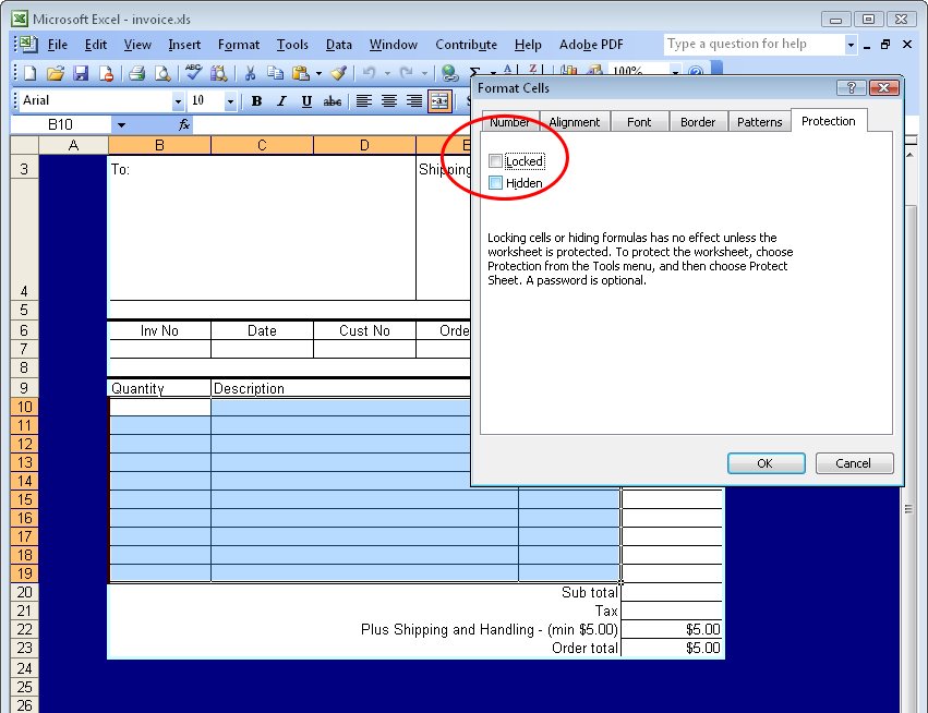
If you haven't protected a workbook before you may find the process of doing so a little confusing. First you hage to unlock the cells that you want your user to have access to. These will be the cells that they can make changes to such as cells they need to add data to. You do this because all cells, by default, are locked against changes.

Select the cells the user should be able to change and choose Format > Cells > Protection and disable the locked checkbox.

Now choose Tools > Protection > Protect Sheet and, if desired, enter a password that will be required to unprotect the sheet so that it cannot be unprotected without permission. Click Ok and the cells that are locked — in other words everything that you didn’t unlock — will now be protected so that the user cannot change them.

The only cells your user will have access to are those that you unlocked for them to use. In this way, you can protect your formulas so that users cannot change them or overwrite them with fixed values which would render the worksheet potentially inaccurate.

Excel - print charts in black and white

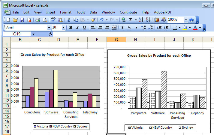
Although your Excel chart might look great in color on the screen, if you're printing to black and white or printing in color and planning to reproduce the charts in black and white you might be disappointed with the final result. Light green, light blue and light orange all look very different on the screen but are indistinguishable in black and white.

So, when your chart is destined for reproduction in black and white, set it up so it is guaranteed to be readible. To do this, select each series or data point by clicking on it, right click and choose Format Data Series (or Format Data Point)> Patterns tab > Fill Effects > Pattern and use a grey or a black and white pattern. Repeat for all the series and save before printing. The chart is guaranteed to look good when printed.

Excel - calculating workdays with Networkdays

Excel has lots of very cool functions for doing all sorts of calculations. One of these is the NETWORKDAYS function.

You can use it to calculate the number of days between two dates taking into account holidays.

Start by placing the dates for the holidays in a range of cells across a row or down a column. Select this range and name it holidays using Insert > Name > Define.

The function calculates the number of workdays between two dates so place one, for now, in cell A1 and the other in A2. This function will calculate the days between the dates in cells A1 and A2 taking into account the holidays listed in the range called Holidays:

=NETWORKDAYS(A1,A2,Holidays)

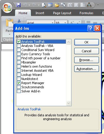
If the NETWORKDAYS function returns an error make sure that you have the Analysis Toolpak installed as this function is stored in this toolpak. To install it in Excel 2003 choose Tools > Add-ins and enable its checkbox. In Excel 2007, click the Microsoft Office Button > Excel Options > Add-Ins and from the Manage list choose Excel Add-ins and click Go. In the Add-Ins Available list enable the Analysis ToolPak checkbox and click OK.

Solving printing problems in Excel

I've seen adults brought almost to tears over printing worksheets. Big worksheets consume lots of paper and when things go wrong they do so in a spectacularly wasteful way. Sometimes the best you can do is hit the printer Off switch to at least achieve a short term solution to the problem. A longer term solution is to understand how you can control what is printed and that's what I'll cover this month. I'll look at the basics of printing a worksheet and then explore some more advanced options which offer better control over your printouts.

Troubleshooting problems
When you choose File > Print or click the Print button in Excel, the program determines what to print and does so. By default it prints everything on the currently active sheet. So, if you have a small set of data in the top corner of the worksheet and have accidentally typed something into a cell way below this (even if it is just a single space), you'll get your data and everything else between this and the one cell with the mistaken entry printed. It could be pages and pages of blank paper – or lined paper if you have gridlines enabled and it's perilously hard to track what went wrong.

You can see ahead of time that you're about to have problems if you use the Print Preview tool. When the Next button is visible there are more pages to print than the one you can see. Of course, you should take care to never place a space in a cell. If you need to remove the cell's contents, click in the cell and press Delete never use the spacebar.

If you can't find the problem cell to delete it, you can try to fix the problem by deleting all the rows below your data and all the columns to the right of it and try again. In the long term this will avoid the problem happening when you print the workbook again next time. If this is a one off worksheet, you can select the area to print before printing it. Drag over the area to print and choose File > Print (don't click the Print button on the toolbar as it prints the entire sheet regardless of what is selected). When the Print dialog appears, click Selection so only the selection will be printed.

Adding Page Breaks
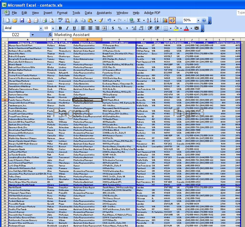
To preview the page breaks on the worksheet to see where the data will be broken up into individual pages, choose View > Page Break View. Lines will appear on the screen indicating where the page breaks are. You can change these by adding your own manual page breaks but you have to do this inside the current page breaks – for example you can add a break inside a page but you can't configure a page to be longer or wider using this method.

To add a manual page break, click to select the entire column or row where the break should appear and choose Insert > Page Break – the page break will be added to the immediate left of this column or immediately above the row. You can also click a cell and choose Insert > Page Break and a page break will be added above and to the left of that cell. When in Page Break View, not only are page breaks visible on the screen, you can also move them by dragging on them with your mouse.



Headings on all worksheet pages
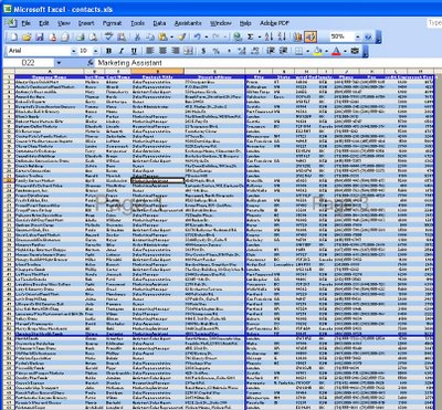
Another issue when printing is that as soon as a sheet prints on more than one sheet of paper, the column headings or row headings appear on the first page but won't appear on the other pages. This makes the data on the second and subsequent pages almost impossible to understand unless they're taped together to form a single large sheet.

To avoid this, configure Excel to print column and row headings on every page of your printout. Choose File > Page Setup > Sheet tab and click in the 'Rows to repeat at top' box – type the row letters in the form $1:$1 (to print only the first row) or $1:$2 for the second etc.. If preferred, you can click the Collapse Dialog button to hide the dialog while you select the rows to use. Likewise you can set the columns that contain the row titles – generally these are in column A and you specify it in the 'Columns to repeat at left' box with an entry like $A:$A to use just the first column or $A:$B for the first two, etc..

More printing controls
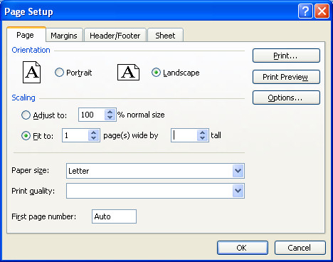
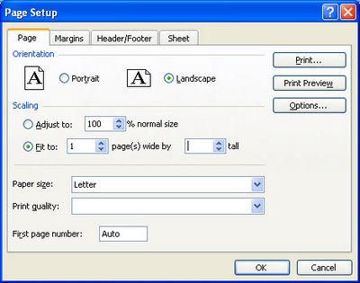
When printing a worksheet that is wider than it is tall, you can print onto paper in landscape orientation to take advantage of the dimensions of the paper. To do this, choose File > Page Setup > Page tab and select Landscape. At the same time, make sure you’ve selected Letter or A4 paper depending on what you're using as each has different dimensions.

Shrink to fit
When you have a worksheet that is just too large to print on a single piece of paper you can shrink it to fit on a single sheet by choosing File > Page Setup > Print tab and click the 'Fit to 1 page(s) wide by 1 page tall' option and it will be reduced to fit on a single sheet.

If your data is very long and you want to print it one page wide but on many pages long you can use the same option – in this case set it so it reads 'Fit to 1 page(s) wide' and delete the entry in the second box – Excel will constrain the width to a single page but print on as many sheets as are needed length-wise.

The same can be done for a worksheet that is wider than it is tall – remove the entry from the first box so it reads 'Fit to page(s) wide by 1 page tall'. Of course, you can also set the value to 2 pages wide or tall or more as required.

When a worksheet will print over multiple sheets in both directions the order in which the sheets are printed may be important. You have two choices – you can have Excel print down the left side of the worksheet first and then across to the next series of pages to the right or you can have it print the width of the worksheet first then the pages below this. This order can be controlled using File > Page Setup > Sheet tab – and select either 'Down, then over' (the default) or 'Over, then down'.

Excel: Open multiple workbooks

If you're like me, you will open Excel in the morning and then open a series of workbooks that you work on each day. You can save time in finding and loading these files by creating an Excel Workspace.

To do this, open all the workbooks you want to have opened each time you launch Excel and then save them as a Workspace file by choosing File > Save Workspace and type a name for the file. Click Save and you can then open all the workbooks at one time by opening the Workspace file. Of course, if you just want to open a single file you can open it as normal.

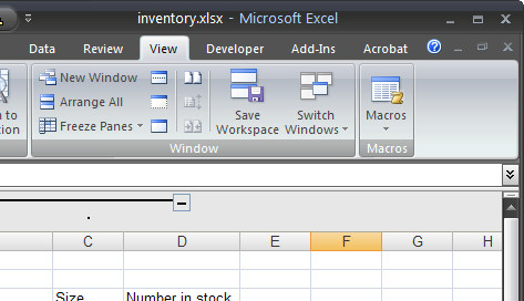
In Excel 2007 - find the Workspace feature by choosing View > Window > Save Workspace.

Another alternative for opening files automatically when Excel opens is to save the file to the XLStart folder - when you do this, the file is opened every time Excel launches.

Excel Change the Default font

If the default font that Excel 2003 uses for all new worksheets doesn't suit your needs - change it by selecting Tools > Options > General tab and set the Standard font and Size to your preferred choice and choose Ok.

In future, all new workbooks you create will be set by default to this font although those you have previously created will remain unchanged.

If you're using Excel 2007 and you don't fancy the new Calibri font, click the Office button, choose Excel Options and click the Popular group. From the Use this font dropdown list choose the font to use for your new worksheets and click Ok. You'll need to close Excel and restart it for the new font change to be in force.

Excel - reuse chart formats

You've gone to all the trouble to format a chart nicely and you'd like to reuse the format again some time in the future. Instead of recreating the format each time, save it so you can apply it with a single click.

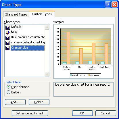
In Excel 2003, right click your chart and choose Chart Type > Custom Types tab and click the User-Defined button. When you do this an Add button appears - click it and type a name and description for your chart when prompted to do so. Click Ok twice when you are done.

Now, in future, when you create a chart you can select this format from the Chart Wizard options or apply it to an existing chart by selecting the chart, right click and choose Chart Type > Custom Types and click User-defined. Select your format and click OK to apply it to the chart.

One word of warning, for some reason, Excel includes chart titles as a format so you'll lose your existing chart title if you have one when you apply the new format to it. It's not a big deal but it helps to know that it's going to happen.

Excel 2007 makes Lovely Lists

Lists were a big addition to Excel 2003 as they allowed you to work with list data in Excel more easily than ever before. One key plus was that they let you create charts that expanded automatically as the data in the list grew. This was something you simply couldn't do before very easily.

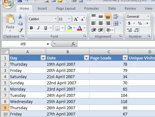
Now in Excel 2007 lists are called tables and they are simple to create using the Format As Table option on the Home tab on the Ribbon. One gotcha is that you shouldn't use a table format if you don't want to create a list, instead use the much more cumbersome and much less pretty Cell Styles options.

When you create a list you automatically get Filter buttons for the list. If you don't like or want them, disable them by clicking to disable the Filter button on the Data tab - just make sure your cell pointer is somewhere in the list when you do this. Like in Excel 2003, if you create a chart based on your table, it expands when you add new data to it.

Multiple Paragraphs of text in an Excel cell

Multiple paragraphs of text in an Excel cell sound good, they look good but how the heck do you create them? If you press the Enter key you enter the current text into the cell and move away from it - obviously, pressing the Enter key isn't the answer.

The solution is to press Alt + Enter to create a new line of text in the current cell. Do this as often as you need to. You might have to make the row taller to fit the text if Excel doesn't make the adjustment for you.

Freeze your titles

When a worksheet exceeds one screen it can be difficult to work as the title row disappears off the screen. Solve this by freezing the titles in place so they don't move but you can still move around your worksheet - it's the best of both worlds.

To do this, place your cell pointer below and to the right of the row and column containing your column and row titles. Not choose Windows > Freeze Panes to fix these rows. These titles are saved with your worksheet.

If you need to undo them at a later date, choose Window > Unfreeze Panes to undo the effect.

Selecting chart elements in Excel 2007

It used to be easy to know what part of a chart you had selected in Excel 2003 - you just read the name off the left hand side of the Formula Bar.

Look in vain for this same feature in Excel 2007. Click anything on the chart and the formula bar just says Chart 1 - like duh! I know I have the chart selected it's the element on it that I'm interested in.

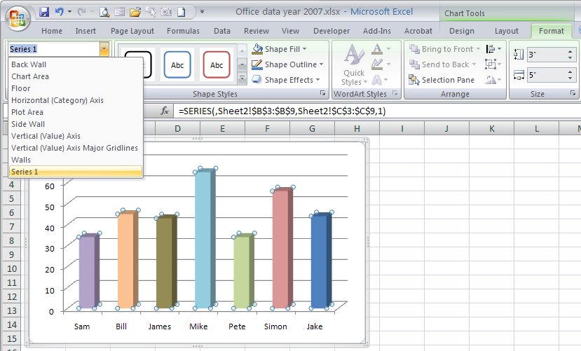
The solution is the new Chart Element tool. Click the chart to select it, choose Chart Tools > Format on the ribbon and in the top left corner is the Chart Element list. Not only will it tell you what you have selected on the chart but it's a dropdown list of names of various chart elements. Click one and that portion of the chart is selected automatically.

It's a handy new tool, I'd just like the benefits of the features from Excel 2003 and 2007 blended into one.. call me fussy.

Do You Undo?

This post is subtitled Undos that Do and Those that Don't

If you're using Excel 2003 or earlier, you have a big problem with the Undo command, you see much of the time, it plain doesn't work.

Curious? Try this: open an Excel file, make some changes to it (minor however, you won't be able to undo these however much you think you can). Check the Undo button - it is enabled. Save the file. Now check the Undo button again. Yikes, it's now disabled. You see, after you save a file in Excel 2003, all the Undo steps are removed - no more Undo. It pays to know this is how it works.

In Excel 2007, things are much better, and the Undo retains the changes even after you have saved the file. Much nicer behavior.

Take a snap - Excel 2003 and earlier.

Need a copy of part of an Excel worksheet? Too easy!

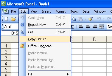
You can take a picture of a range in Excel and, for example, insert into Word as a picture or place it an image in another area on a workbook. To do this, first select the area to snap and hold Shift as you open the Edit menu. Choose Copy Picture, select As shown on screen or As shown when printed and click Ok.

Now go ahead and paste the image wherever you desire. This Shift + Edit menu option also works for copying a clip art or other type of image inserted into an Excel workbook.

Error Checking in Excel

Chasing problems in Excel worksheets is a major pain. It helps to create them accurately in the first place but when you're trying after the fact, to find problems, Excel has some tools that can help. One of these is the often overlooked Go To option.

Go To can find formulas that vary from those in the cells that surround them. This can help you find formula errors which would otherwise be difficult to locate.

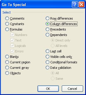
So, for example, if you have a column of cells which should all contain the same formula you can check to make sure they are written the same way by selecting the cells and choose Edit, Go To, Special, Column Differences (in Excel 2007, from the Home tab select Find & Select, Go To Special and then click Column Differences). Any cells which contain a formula that relates to a different series of cells to those in the active cell will be selected so you can check them. The Row Differences option does the same thing for rows of cells.

View formulas in Excel

If you've ever wanted to view your formulas in an Excel worksheet, perhaps because you suspect one has been overwritten by data or you need to troubleshoot something press CONTROL + ~ to display formulas so you can troubleshoot or debug them. Press the same keystroke again to return to your regular view of your worksheet.

If you select a cell with a formula in it before you press CONTROL + ~ you will see not only the worksheet formulas but also all the precedents to the formula in the current cell.

How old are you?

I know.. it's none of my business, but sometimes you wonder, don't you, just how old you are in days? If this question consumes your waking hours, put the calculator away and crank up Excel.

Excel's Datedif function, while not documented, calculates the difference between two dates in a number of formats; days, months or years. The syntax of the function is: =datedif(start date,end date,units to return). The units must be provided by a quoted string in the format: "y" - full years, "m" - full months, "d" - full days, "md" - full days in excess of the last full month, "ym" - full months in excess of the last full year and "yd" - full days in excess of the last full year.

So, for example, this formula determines the number of days between the dates in cells B6 and C6: =DATEDIF(B6,C6,"d"). Type your birthday and today's day in the cells and you'll know immediately how old you are in days..

Excel Fill Options

You probably already know that you can fill a series of Excel cells by entering the first two numbers in a series and then select the two cells and drag on the marker in the bottom right corner of the selection. Excel fills the selected cells with the next numbers in the series. to find more fill options, including the ability to copy the series rather than filling it, select the cells but use the right mouse button to do the dragging. If you're filling dates you'll get options like Fill Weekdays and Fill Months - that let you control the fill series that Excel creates for you.